2020-11-22

数字图像处理实验：直方图和频域滤波

Starry, starry night
Paint your palette blue and grey
Look out on a summer's day
With eyes that know the darkness in my soul
Shadows on the hills
Sketch the trees and the daffodils
Catch the breeze and the winter chills
In colors on the snowy linen land

点此下载代码和示例图片

1. 代码组织结构和使用说明

1.1 代码组织结构

本次实验编写的程序为 C++编写的 Linux 环境下命令行可执行程序，而非 PPT 上说的早就过时的 Windows MFC程序。

ps.cpp：主程序代码（our own PhotoShop）
bmp.cpp和bmp.hpp：封装对 BMP 图像的处理操作
color.cpp和color.hpp：封装对色彩空间的操作
fft.cpp和fft.hpp：图像的快速傅里叶变换和频率域滤波操作
utils.cpp和utils.hpp：通用函数

1.2 编译

使用已写好的Makefile文件编译，编译后生成ps二进制文件，通过命令行输入输入和输出的文件路径，以及对文件进行处理的参数。

由于本次实验使用了fftw3快速傅里叶变换库，因此在编译前，应确保安装了该库：

sudo apt install libfftw3-dev

之后编译时，应使用

1	`-lfftw3 -lm`

参数进行链接。在 Makefile 中已经实现。

1.3 使用说明

本程序通过命令行指定路径读取 BMP 文件，并可指定参数，进行对应的图像处理。参数可以叠加，这时将依次执行处理操作。使用说明如下：

Usage:          ./ps input_img [-d|-l|-h|-e|-n|-b|-o]
Pamameters:
-d              Show DFT Transform spectrum
-l filter_size  Gaussian low pass filter
-h filter_size  Gaussian high pass filter
-e              Equalization histogram of input image
-n ref_img      Normalization histogram of input image with reference image
-b threshold    Binarize image into 2-color with given threshold
-o output_img   Output image

例如，对图像test.bmp进行低通滤波后再均衡化输出到test_out.bmp，可使用

./ps test.bmp -l 20 -e -o test_out.bmp

2. BMP 图像的格式和读写

在bmp.hpp中定义 BMP 类：

// BMP Read & Write & Manipulate Class
class BMP
{
private:
    Header header;  // BMP Header
    Color *px;      // pixels
    Color *colors;  // color plate
    int colors_num; // size of color plate
    int padding;    // padding bytes of each line
    int *his;       // V channel histogram

    Color get_color(int index);
    int find_color(Color &px);
    void read1(FILE *fp);
    void read4(FILE *fp);
    void read8(FILE *fp);
    void read24(FILE *fp);
    void write1(FILE *fp);
    void write4(FILE *fp);
    void write8(FILE *fp);
    void write24(FILE *fp);
    void to1();
    void to8();
    void to24();
    void hsv();
    void rgb();

public:
    BMP(const char *filename);
    ~BMP();
    void info();
    void dft();
    void low_pass_filter(double filter_size);
    void high_pass_filter(double filter_size);
    void equalize();
    void normalize(int *his);
    void binarize(int threshold);
    int *histogram();
    void write(const char *filename);
};

此后对 BMP 的文件处理均围绕该类展开。其中

header：存放头部信息
px：存放像素数据
colors：存放调色板信息
colors_num：调色板个数
padding：每行为 4 字节对齐填充的字节数（后文会提到）
his：存放直方图信息

后续的这些函数和变量均会有说明或在注释中体现，不再赘述。

2.1 BMP 文件头格式

在bmp.hpp中定义Header结构体，采用 1 字节对齐。并使用cstdint库确保整数位数的一致：

#pragma once
#pragma pack(push, 1)
// BMP File Header
struct Header
{
    std::uint16_t bmp;              // Magic number for file
    std::uint32_t file_size;        // Size of file
    std::uint16_t reserved_1;       // Reserved
    std::uint16_t reserved_2;       // Reserved
    std::uint32_t offset;           // Offset to bitmap data
    std::uint32_t header_size;      // Size of info header
    std::uint32_t width;            // Width of image
    std::uint32_t height;           // Height of image
    std::uint16_t plans;            // Number of color planes
    std::uint16_t depth;            // Number of bits per pixel
    std::uint32_t compression;      // Type of compression to use
    std::uint32_t image_size;       // Size of image data
    std::uint32_t ppm_x;            // X pixels per meter
    std::uint32_t ppm_y;            // Y pixels per meter
    std::uint32_t colors;           // Number of colors used
    std::uint32_t colors_important; // Number of important colors
};
#pragma pack(pop)

其中值得关注的点是

offset：存放像素区域的从文件开始处的偏移量
width：图像宽度
height：图像高度
depth：位深度，即一个像素占几个 bit，决定了这张图是几色的图：2 色图为 1，16 色图为 4，256 色图为 8，真彩色图为 24
colors：调色板颜色数。大多数情况下，这个数字被设置为 0，则实际调色板个数由位深度决定：
位深度为 1 的默认有 2 个调色板
位深度为 4 的默认有 16 个调色板
位深度为 8 的默认有 256 个调色板
位深度为 24 的没有调色板

2.2 BMP 调色板区域格式

每个调色板由 4 个字节组成，依次为 R、G、B、保留。相邻两个调色板之间是连续的。可在color.hpp定义Color结构体：

// Color Platte
struct Color
{
    bool type = false; // false for HSV, true for RGB
    std::uint8_t r;    // Red
    std::uint8_t g;    // Green
    std::uint8_t b;    // Blue
    std::uint8_t a;    // Reserved
    void hsv();
    void rgb();
};

此处考虑到了之后的色彩空间转换，提供了两个转换函数和一个type标识符。因此建一个Color数组，即可表示调色板。并且编写了调色板数组中的下标和对应Color结构体映射的两个函数get_color和find_color，用于之后的文件读写：

// Get a color from color table
// index: color index
Color BMP::get_color(int index)
{
    Color color;
    color.r = colors[index].r;
    color.g = colors[index].g;
    color.b = colors[index].b;
    color.a = colors[index].a;
    return color;
}

// Find a color index in color table
// color: color, which index is to be found
int BMP::find_color(Color &color)
{
    for (int i = 0; i < colors_num; i++)
    {
        if (color.r == colors[i].r && color.g == colors[i].g &&
            color.b == colors[i].b && color.a == colors[i].a)
            return i;
    }
    return -1;
}

2.3 BMP 数据区域格式

数据区域，按照从左至右，从下往上的顺序存储。从左到右为一行。每行之间的像素均相邻，但是在行尾会有一定数量的 0 字节填充，使每行的长度为 4 字节的整数倍，也叫做4 字节对齐。因此不能想当然的二重循环直接读写，应该先计算偏移量：

padding = (4 - (((header.width * header.depth + 7) / 8) % 4)) % 4;

由于每次读写的最小单位是 1 字节，因此对于位深度小于 8 的，应进行相应的计算处理：

对于 2 色图：1 个字节中的 8 个 bit 表示 8 个像素，且低位的在先，高位的在后。每个 bit 的值 0 或 1 代表其在调色板中的颜色索引
对于 16 色图：1 个字节中的 8 个 bit，分成两组 4bit，表示两个像素。且低位的 4bit 表示第一个像素，高位的 4bit 表示后面的第二个像素。这里 4bit 对应的数值也是调色板中的颜色索引
对于 256 色图，1 个字节就是 1 个像素，且这里的值也是表示调色板中的颜色索引，而非 0~255 灰度值
对于真彩色图，3 个字节是 1 个像素，分别按照 B、G、R 通道排列。其中每个通道对应的 1 个字节的内容代表该通道的像素值 0~255（彩色图没有调色板了）

2.4 BMP 图像的读写

写的函数和读类似，以读来举例。在 BMP 类中，定义构造函数即为读函数，接收一个字符串参数，指向文件名：

// Constructor
// filename: BMP image file
BMP::BMP(const char *filename)
{
    uint8_t byte;
    FILE *fp;

    // File header
    if ((fp = fopen(filename, "rb")) == NULL)
        throw_ex("fopen");
    if (fread(&header, sizeof(Header), 1, fp) < 0)
        throw_ex("fread");

    // Color plates
    colors_num = (header.colors == 0 && header.depth != 24) ? (1 << header.depth) : header.colors;
    colors = new Color[colors_num];
    for (int i = 0; i < colors_num; i++)
    {
        fread(&byte, 1, 1, fp);
        colors[i].r = byte;
        fread(&byte, 1, 1, fp);
        colors[i].g = byte;
        fread(&byte, 1, 1, fp);
        colors[i].b = byte;
        fread(&byte, 1, 1, fp);
        colors[i].a = byte;
    }

    // Pixels
    padding = (4 - (((header.width * header.depth + 7) / 8) % 4)) % 4;
    px = new Color[header.width * header.height];
    switch (header.depth)
    {
    case 1:
        read1(fp);
        break;
    case 4:
        read4(fp);
        break;
    case 8:
        read8(fp);
        break;
    case 24:
        read24(fp);
        break;
    }
    fclose(fp);
    his = new int[256];
}

依次读取文件头、读取调色板、读取像素。读取文件头后，还要通过文件头的信息计算调色板个数color_num和每行像素对齐追加的字节数padding。之后，根据不同的位深度情况，调用不同的读取函数。以read4举例：

// Read 4-bit BMP file
// fp: file pointer
void BMP::read4(FILE *fp)
{
    uint8_t byte;
    fseek(fp, header.offset, SEEK_SET);
    for (int i = header.height - 1; i >= 0; i--)
    {
        for (int j = 0; j < header.width; j += 2)
        {
            if (fread(&byte, 1, 1, fp) < 0)
                throw_ex("fread");
            px[header.width * i + j] = get_color(byte & 0x0F);
            px[header.width * i + j + 1] = get_color(byte >> 4);
        }
        fseek(fp, padding, SEEK_CUR);
    }
}

首先通过fseek跳到数据区，之后由于 BMP 格式是从下往上，但是实际在数字图像处理中，一般让 $x$ 轴从上往下，因此对于行逆序读取。在读取像素时，由于 4 为图，一个字节有两个像素，因此要讲这两个像素通过位运算拆分，依次写入px数组。并且要在每读完一行后跳过padding区域。

写操作也类似。对于位深度为 1 的 2 色图，写操作如下：

// Write 1-bit BMP file
// fp: file pointer
void BMP::write1(FILE *fp)
{
    uint8_t byte;
    fseek(fp, header.offset, SEEK_SET);
    for (int i = header.height - 1; i >= 0; i--)
    {
        for (int j = 0; j < header.width; j += 8)
        {
            byte = 0;
            for (int k = 0; k < 8; k++)
                byte += find_color(px[i * header.width + j + k]) << (7 - k);
            fwrite(&byte, 1, 1, fp);
        }
        fwrite("\0", 1, padding, fp);
    }
}

为了之后的部分操作的方便，可以将图像统一转换为 24 位彩色存储，因此编写了to24函数，其无非就是调整头部结构体中的图像大小、偏移量、调色板个数和位深度信息：

// Convert current BMP image into 24-bit
void BMP::to24()
{
    header.offset = 54;
    header.depth = 24;
    padding = (4 - (((header.width * header.depth + 7) / 8) % 4)) % 4;
    header.image_size = (header.width * 3 + padding) * header.height;
    header.file_size = header.offset + header.image_size;
    colors_num = 0;
}

同时为了二值化和灰度化处理方便，也编写了将图片转为 1 位图进行存储的to1函数和转为 256 色灰度图存储的to8函数：

// Convert current BMP image into 1-bit
void BMP::to1()
{
    header.offset = 62;
    header.depth = 1;
    header.colors = 0;
    padding = (4 - (((header.width * header.depth + 7) / 8) % 4)) % 4;
    header.image_size = ((header.width + 7) / 8 + padding) * header.height;
    header.file_size = header.offset + header.image_size;

    delete[] colors;
    colors_num = 2;
    colors = new Color[colors_num];
    colors[0].r = 0;
    colors[0].g = 0;
    colors[0].b = 0;
    colors[0].a = 0;
    colors[1].r = 255;
    colors[1].g = 255;
    colors[1].b = 255;
    colors[1].a = 0;
}

// Convert current BMP image into 8-bit
void BMP::to8()
{
    header.offset = 1078;
    header.depth = 8;
    header.colors = 0;
    padding = (4 - (((header.width * header.depth + 7) / 8) % 4)) % 4;
    header.image_size = (header.width + padding) * header.height;
    header.file_size = header.offset + header.image_size;

    delete[] colors;
    colors_num = 256;
    colors = new Color[colors_num];
    for (int i = 0; i < colors_num; i++)
    {
        colors[i].r = i;
        colors[i].g = i;
        colors[i].b = i;
        colors[i].a = 0;
    }
}

3. 直方图均衡化和规格化

由于所有的像素数据都存放在px数组中，因此后续的图像处理操作均可围绕px数组，以及头部信息中的长和宽header.width、header.height展开。

此处的均衡化和规格化均只考虑灰度值的分布在 0~255 之间的情况

3.1 直方图数组获取

直方图即灰度值的统计分布。横轴为灰度值，纵轴为该灰度值下的像素个数，因此编写histogram函数获取直方图数组：

// Calculate image histogram
int *BMP::histogram()
{
    hsv();
    for (int i = 0; i < 256; i++)
        his[i] = 0;
    for (int i = 0; i < header.width * header.height; i++)
        his[px[i].b]++;
    rgb();
    return his;
}

存放在histogram数组中。

3.2 灰度图均衡化

根据《数字图像处理》教材公式，设 $m a p [i]$ 为原先的灰度值为 $i$ 的像素，均衡化后应该变成的灰度值。则

m a p [i] = \frac{255}{w i d t h \times h e i g h t} \sum_{k = 0}^{i} h i s t o g r a m [k]

即对之前所有的直方图分布做了一个平滑。之后，遍历每个灰度值 $i$ ，令 $i \leftarrow m a p [i]$ ，即可完成均衡化。可编写部分代码如下（以 B 通道为例）：

// Histogram equalization
void BMP::equalize()
{
    ...
    int *map = new int[256];
    int sum;
    double size = header.width * header.height;
    // Value Channel
    sum = 0;
    for (int i = 0; i < 256; i++)
    {
        sum += histogram[i];
        map[i] = (int)round(255 * sum / size);
    }
    for (int i = 0; i < size; i++)
        px[i].b = map[px[i].b];
    for (int i = 0; i < colors_num; i++)
        colors[i].b = map[colors[i].b];
    ...
    calc_histogram();
    delete[] map;
}

注意到调色板的颜色也要均衡化，以确保保存时可以对应。效果如下图右上角所示。

3.3 彩色图均衡化

但是，上面只是针对灰度图，RGB 三通道的值相同的情况。对于彩色的图，我们首先想到的是分开处理三个通道，分别均衡化。但是这样做会导致颜色不一致的问题，如右下角所示：

因为均衡化的目的是均衡亮度，而 RGB 三个通道没有一个通道能独自体现亮度，因此需要先进行色彩空间转换。这里选择将 RGB 转换成 HSV，其中 V 通道表示亮度。

在color.cpp中编写了两个通道互相转换的函数：

// RGB to HSV in-place
void Color::hsv()
{
    if (type)
        return;
    double R, G, B, H, S, V;
    R = r / 255.0;
    G = g / 255.0;
    B = b / 255.0;
    double X_max = max(R, max(G, B));
    double X_min = min(R, min(G, B));
    double C = X_max - X_min;
    V = X_max;
    if (C == 0)
        H = 0;
    else if (V == R)
        H = 60 * (0 + (G - B) / C);
    else if (V == G)
        H = 60 * (2 + (B - R) / C);
    else
        H = 60 * (4 + (R - G) / C);
    if (V == 0)
        S = 0;
    else
        S = C / V;
    r = (uint8_t)round(H / 2);
    g = (uint8_t)round(S * 255);
    b = (uint8_t)round(V * 255); // H/S/V both in 0~255
    type = true;
}

// HSV to RGB in-place
void Color::rgb()
{
    if (!type)
        return;
    double R, G, B, H, S, V;
    H = (r * 2) / 60.0;
    S = g / 255.0;
    V = b / 255.0;
    double C = V * S;
    double X = C * (1 - fabs(fmod(H, 2) - 1));
    double M = V - C;
    if (0 <= H && H <= 1)
        R = C, G = X, B = 0;
    else if (1 < H && H <= 2)
        R = X, G = C, B = 0;
    else if (2 < H && H <= 3)
        R = 0, G = C, B = X;
    else if (3 < H && H <= 4)
        R = 0, G = X, B = C;
    else if (4 < H && H <= 5)
        R = X, G = 0, B = C;
    else if (5 < H && H <= 6)
        R = C, G = 0, B = X;
    else
        R = 0, G = 0, B = 0;
    r = (uint8_t)round((R + M) * 255);
    g = (uint8_t)round((G + M) * 255);
    b = (uint8_t)round((B + M) * 255);
    type = false;
}

采用了 in-place 模式，原来的 R、G、B 分别对应 H、S、V。且由于 HSV 通道中，H 的值通常是 0-360，S 的值和 V 的值通常是 0~100，这里做了缩放处理，统一规定在 0-255 区间内。

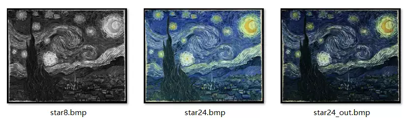
有了通道转换后，对于彩色图像的均衡化，只需在计算前换成 HSV 空间，然后对 V 通道均衡化，计算后再换回 RGB 空间即可。效果如下图所示：

3.4 直方图匹配

同样，这里针对 V 通道进行说明（灰度图的 V 通道对应的就是其灰度值）。由课本公式，设 $m a p [i]$ 为原先的灰度值为 $i$ 的像素，均衡化后应该变成的灰度值； $h i s t o g r a m_{2}$ 为被逼近的直方图。则在先对图像进行均衡化后，有

g [i] = 255 \times \sum_{k = 0}^{i} h i s t o g r a m_{2} [k]

m a p [i] = g^{- 1} [i]

由于 $g [i]$ 显然单调递增，因此通过简单的二分查找就能获取到 $g^{- 1} [i]$ 的值。可使用 C++algorithm库中的lower_bound函数实现。编写程序如下：

// Histogram normalization
// his: new distribution of histogram
void BMP::normalize(int *his)
{
    equalize();
    hsv();
    int *g = new int[256];
    int *map = new int[256];
    int sum;
    double size = header.width * header.height;
    // We process only value channel
    sum = 0;
    for (int i = 0; i < 256; i++)
    {
        sum += his[i];
        g[i] = (int)round(255 * sum / size);
    }
    for (int i = 0; i < 256; i++)
        map[i] = lower_bound(g, g + 256, i) - g;
    for (int i = 0; i < size; i++)
        px[i].b = map[px[i].b];
    rgb();
    calc_histogram();
    delete[] g;
    delete[] map;
}

用 256 色的灰度图的直方图分布来规格化彩色图的直方图，效果如右侧star24_out.bmp所示：

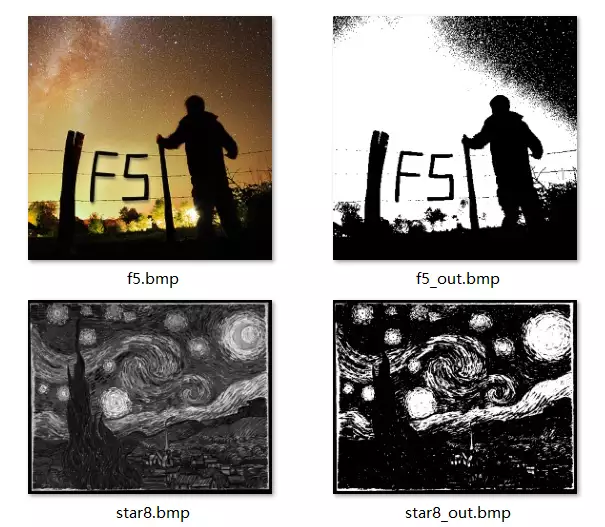
3.5 图像二值化

我们可以根据直方图的分布，将图像进行二值化。事实上，只需根据 V 通道的值是否超过设定的阈值，决定该像素是 0 或 1 即可。同时，为了节约空间，可将二值化之后的图转成 2 色图存储，因此用到之前的to1函数：

// Binaize an image into black and white
// threshold: Value channel threshold
void BMP::binarize(int threshold)
{
    hsv();
    for (int i = 0; i < header.height; i++)
        for (int j = 0; j < header.width; j++)
            if (px[i * header.width + j].b > threshold)
            {
                px[i * header.width + j].b = 255;
                px[i * header.width + j].g = 255;
                px[i * header.width + j].r = 255;
            }
            else
            {
                px[i * header.width + j].b = 0;
                px[i * header.width + j].g = 0;
                px[i * header.width + j].r = 0;
            }
    to1();
}

分别对彩色图和 16 色图采用 100 的阈值进行二值化，效果如下图所示：

4. FFT 和频率域滤波

这里均借助fftw3库实现 FFT 算法。需通过以下命令在 Linux 下安装：

sudo apt install libfftw3-dev

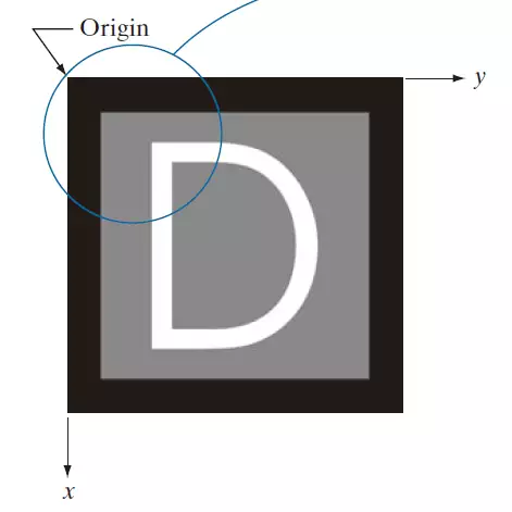
4.1 图像约定

对于图像坐标，这里按照课本相同的约定，原点在左上角， $x$ 轴为高度，程序中用i表示， $y$ 轴为宽度，程序中用j表示。

频谱展示部分，对于灰度图来说，可以直接用灰度值进行 DFT，但是对于彩色图像，这里也是将其转换到 HSV 空间，并用 V 通道计算 DFT。

但是对于频率域滤波部分，这时候对于彩色图像，是分成三个通道，分别进行 DFT、滤波、IDFT 计算。

4.2 二维 DFT 频谱展示

4.2.1 代码框架

根据 fftw 的文档，使用步骤的代码框架如下图所示：

#include <fftw3.h>
...
{
    fftw_complex *in, *out;
    fftw_plan p;
    ...
    in = (fftw_complex*) fftw_malloc(sizeof(fftw_complex) * N);
    out = (fftw_complex*) fftw_malloc(sizeof(fftw_complex) * N);
    p = fftw_plan_dft_1d(N, in, out, FFTW_FORWARD, FFTW_ESTIMATE);
    ...
    fftw_execute(p); /* repeat as needed */
    ...
    fftw_destroy_plan(p);
    fftw_free(in); fftw_free(out);
}

先通过fftw_malloc创建输入和输出的复数数组存储空间
之后通过fftw_plan*系列函数创建计算计划
之后通过fftw_execute执行计算
最后通过destory_plan和fftw_free释放计划和复数数组的空间

其中fftw_complex表示复数，实际上每一个fftw_complex是一个double [2]，其中下标 0 表示实部，下标 1 表示虚部。

4.2.2 格式转换

为了实现我们的频谱展示，首先需要将px数组转为fftw_complex数组。这里可以简单的将实部赋值。但是这样做的后果是输出的频谱原点和图像一样在左上角。如果想要输出的频谱原点在图像中心，可以使用书上的结论：

若图像 $f (x, y)$ 的傅里叶变换为 $F (u, v)$ ，则

f (x, y) (- 1)^{x + y} \Leftrightarrow F (u - \frac{h e i g h t}{2}, v - \frac{w i d t h}{2})

因此我们可以在给实部赋值时，顺带乘上 $(- 1)^{i + j}$ ：

in = (fftw_complex *)fftw_malloc(sizeof(fftw_complex) * width * height);
out = (fftw_complex *)fftw_malloc(sizeof(fftw_complex) * width * height);
if (in == NULL || out == NULL)
    throw_ex("fftw_malloc");

for (int i = 0; i < height; i++)
    for (int j = 0; j < width; j++)
    {
        in[i * width + j][0] = px[i * width + j].b * ((i + j) % 2 ? -1 : 1); // Make sure (0, 0) is at the center of the spectrum
        in[i * width + j][1] = 0;
    }

4.2.3 计算 DFT

根据文档，这里需要创建fftw_plan_dft_2d的计划：

p = fftw_plan_dft_2d(height, width, in, out, FFTW_FORWARD, FFTW_ESTIMATE);
fftw_execute(p);

计算后，结果就存放在out内。

4.2.4 频谱可视化

由于计算结果是复数，因此这里和书上一样，使用频谱的模来确定灰度值。并且书上第 268 页（中文版第 155 页）提到，由于频谱强度在不同频率间差异很大，因此可以通过对频谱强度取对数来提升动态范围。

最后，由于实际的灰度值在 0~255 之间，因此需要对灰度值再进行统一的缩放。设频谱图像为 $f^{'} (x, y)$ ，而之前的傅里叶变换结果为 $F (u, v)$ ，则最后的公式如下：

f^{'} (x, y) = r o u n d (\frac{\log (∣ F (x, y) ∣ + 1)}{\max_{0 \leq u < h e i g h t, 0 \leq v < w i d t h} \log (∣ F (u, v) ∣ + 1)} \times 255)

可编写代码如下：

for (int i = 0; i < height; i++)
    for (int j = 0; j < width; j++)
    {
        double re = out[i * width + j][0];
        double im = out[i * width + j][1];
        f_max = max(f_max, log(sqrt(re * re + im * im) + 1)); // use log to enhance low-power freqencies
    }
for (int i = 0; i < height; i++)
    for (int j = 0; j < width; j++)
    {
        double re = out[i * width + j][0];
        double im = out[i * width + j][1];
        uint8_t value = (uint8_t)round(log(sqrt(re * re + im * im) + 1) / f_max * 255); // use log to enhance low-power freqencies
        px[i * width + j].b = value;
        px[i * width + j].g = value;
        px[i * width + j].r = value;
    }

4.2.5 函数原型和测试

将上述计算环节编写为fft_dft函数，原型如下：

// Calculate DFT of an image, and replace its px in-place
// width:  image width
// height: image height
// px:     image pixel data, and after this, its data will be replaced by it's fourier spectrum in grayscale
void fft_dft(int width, int height, Color *px)

之后，在bmp.cpp中调用该函数。由于频谱是灰度图，因此将图像转为 8 位 256 色图减少存储空间：

// Convert image to fourier spectrum of it's V channel
void BMP::dft()
{
    hsv();
    fft_dft(header.width, header.height, px);
    to8();
}

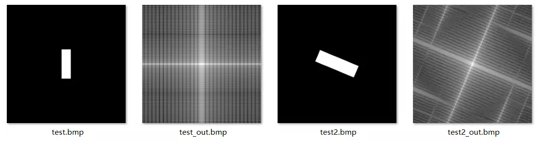
对和课本上类似的图进行测试，效果如下，右侧为这两张图的频谱：

对 Lena 的灰度图和彩色图进行测试，效果如下：

可见灰度图和彩色图的频谱没有什差别，因为彩色图的频谱是用 V 通道计算的。

4.3 频率域滤波

4.3.1 滤波器设计

这里采用课本上的高斯低通滤波器和高斯高通滤波器。滤波器可表示为 $H (u, v)$ ，将 $H (u, v)$ 与频率域的 $F (u, v)$ 相乘，即可得到新的频率域。若设 $s i z e$ 为滤波器尺寸，则

高斯低通滤波器为

H (u, v) = \exp (- \frac{(u - u_{0})^{2} + (v - v_{0})^{2}}{2 \times s i z e})

高斯高通滤波器为

H (u, v) = 1 - \exp (- \frac{(u - u_{0})^{2} + (v - v_{0})^{2}}{2 \times s i z e})

其中

u_{0} = \frac{h e i g h t}{2} v_{0} = \frac{w i d t h}{2}

$s i z e$ 越大，对低通滤波器，表明通过的频率越多，对原图影响的越小；对高通滤波器，表明去除的频率越多，对原图影响的越大。这两个滤波器可编写成以下函数：

// Gaussian low-pass filter
// width:       image width
// height:      image height
// out:         frequency domain data
// filter_size: size of filter in frequecy domain
void gauss_lpf(int width, int height, fftw_complex *out, double filter_size)
{
    double x_center = height / 2.0;
    double y_center = width / 2.0;

    for (int i = 0; i < height; i++)
        for (int j = 0; j < width; j++)
        {
            double d2 = (i - x_center) * (i - x_center) + (j - y_center) * (j - y_center);
            double h = exp(-d2 / (2 * filter_size * filter_size));
            out[i * width + j][0] *= h;
            out[i * width + j][1] *= h;
        }
}

// Gaussian high-pass filter
// width:       image width
// height:      image height
// out:         frequency domain data
// filter_size: size of filter in frequecy domain
void gauss_hpf(int width, int height, fftw_complex *out, double filter_size)
{
    double x_center = height / 2.0;
    double y_center = width / 2.0;

    for (int i = 0; i < height; i++)
        for (int j = 0; j < width; j++)
        {
            double d2 = (i - x_center) * (i - x_center) + (j - y_center) * (j - y_center);
            double h = 1 - exp(-d2 / (2 * filter_size * filter_size));
            out[i * width + j][0] *= h;
            out[i * width + j][1] *= h;
        }
}

4.3.2 IDFT 反变换

当我们通过滤波器得到新的out复数数组后，需要对其进行反变换。由课本公式，我们可以借助 FFT 计算 IDFT：

若

F (u, v) = D F T [f (x, y)]

则

f (x, y) = \frac{1}{w i d t h \times h e i g h t} D F T [\overline{F (u, v)}]

只需取其共轭，并将结果除以图像大小即可。并且由于之前在 DFT 前，将图像乘以了 $(- 1)^{x + y}$ ，因此这里需要再乘 $(- 1)^{x + y}$ 回去，恢复成原来的图像。

并且，这里只需取反变换后的实部部分，即 $r e f (x, y)$ 。可编写代码如下：

for (int i = 0; i < height; i++)
    for (int j = 0; j < width; j++)
        out[i * width + j][1] *= -1;
p = fftw_plan_dft_2d(height, width, out, out, FFTW_FORWARD, FFTW_ESTIMATE);
fftw_execute(p);
for (int i = 0; i < height; i++)
    for (int j = 0; j < width; j++)
    {
        double re = out[i * width + j][0] / (width * height) * ((i + j) % 2 ? -1 : 1);
        if (re > 255)
            re = 255;
        if (re < 0)
            re = 0;
        uint8_t value = (uint8_t)round(re);
        if (c == 0)
            px[i * width + j].b = value;
        else if (c == 1)
            px[i * width + j].g = value;
        else
            px[i * width + j].r = value;
    }

4.3.3 函数原型和测试

将上述步骤编写成fft_dft_idft函数，原型如下：

// Calculate DFT of an image, doing some process in frequency domain, and then IDFT
// width:       image width
// height:      image height
// px:          image pixel data, and after this, it's data will be replaced by it's fourier spectrum in grayscale
// proc:        processing function of frequecy domain
// filter_size: size of filter in frequecy domain
void fft_dft_idft(int width, int height, Color *px, void (*proc)(int, int, fftw_complex *, double), double filter_size)

其中proc即为两种滤波器函数的一个。

在bmp.cpp中调用该函数。由于对 2 色和 16 色图进行滤波后，会产生新的颜色，因此需将其转为 256 色。而彩色图像不变：

// Gaussian low-pass filter
// filter_size: image is blurer if lower
void BMP::low_pass_filter(double filter_size)
{
    if (header.depth <= 8)
        to8();
    fft_dft_idft(header.width, header.height, px, gauss_lpf, filter_size);
}

// Gaussian high-pass filter
// filter_size: image is sharper if higher
void BMP::high_pass_filter(double filter_size)
{
    if (header.depth <= 8)
        to8();
    fft_dft_idft(header.width, header.height, px, gauss_hpf, filter_size);
}

分别对 Lena 的彩色图采用低通滤波，滤波器大小为 2、4、8、16、32：

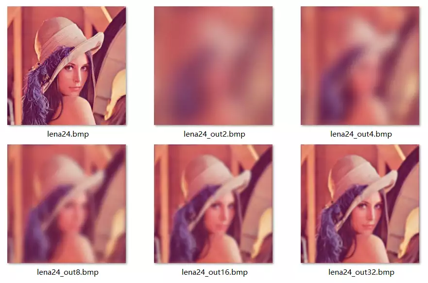
可以发现滤波器大小越小，说明高频部分通过的越少，图像越平滑。再依次采用高通滤波，大小也为 2、4、8、16、32：

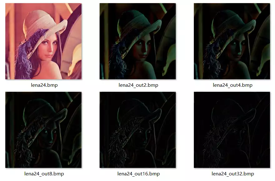
可以发现，滤波器大小越大，说明去除的低频成分越多，边缘越明显。且由于随着低频接近直流的分量去除，图像在平滑处趋近于黑色，在边缘处才有其他颜色。为了增加对比度，接下来将这五张图片进行直方图均衡化：

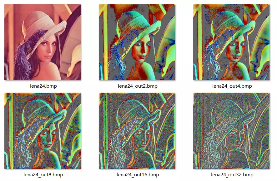
这样可以进一步看出，滤波器大小越大，对边缘特征的提取越明显。

下面是针对测试用图的一些测试，对第一行应用低通滤波，对第二行应用高通滤波，滤波器大小均为 10：

可以发现频谱也有着明显的改变。

对于第二行，由于展示频谱时对范围进行了缩放，因此本来频率强度最高的中心处颜色仍然相同，但可以发现周围的原本颜色深的地方要变得更浅

对于非正方形的图案，算法也有效。以下是对其进行了大小为 10 的低通滤波的结果

点此下载代码和示例图片